Seafood Watch App now available on iPhone and Android

For the tech savvy sea-life eating of the bunch, Seafood Watch has recently gone digital!  

The app provides up-to-date recommendations on ocean-friendly sea-life (seafood and sushi), compatible with iPhones and Androids.

For those of us without apps at our fingertips, Monterrey Bay aquarium still has their traditional pocket-sized list available as a free download, they even make guides by region.  Here's a link to the northeastern US guide (PDF).

Ecosystem cycles, pools, and fluxes

Here are a few resources to help you review some of the Ecosystems concepts covered in this section

Ecosystem Cycling

• Energy Flow Through Ecosystems & Primary Productivity 

• Regulation of Ecosystem Functions, Limiting resources

   

General patterns of energy flow for a) forest, b) grassland, c) plankton, d) stream:

Essentials of Ecology by Townsend et al.

 

Water Cycle

Here's a diagram of the water cycle that you can use to quiz yourself. You may check your answers here.

Useful links:

• Groundwater flow, discharge, & infiltration 
• Follow a drop through the water cycle   
• Water and human health: Water pollution,  Water-related diseases, and Water conservation policies.
• Case study: Chesapeake Bay watershed maps.
  

Biogeochemical cycles

 For a general review of some of these cycles, click here.

Review of greenhouse gases.  This website has a good description of the nitrogen cycle; links on the left sidebar proved more in-depth description.

Nutrient budget components in terrestrial and aquatic ecosystems; Inputs = blue, outputs = black. (Essentials of Ecology by Townsend et al).

Nitrogen Cycle (Learner.org)

Phosphorus cycle (Learner.org)

A comparison of major nutrient cycles (you don't need to know the Sulfur cycle). Source: Townsend et al.

A Dose of Diversity - NWF featured article

In 2010, myself, and my research collaboration was featured in a National Wildlife Federation publication.  

The article entitled "Scientists are discovering that species extinctions fuel the rise and spread of infectious diseases and hinder medical research" is related to our recitation reading by Allan et al.  

To learn more about how diversity may influence vector-borne disease prevalence (and a little about my graduate student research), click on the above link.

NWF 2010 article cover page

April is water awareness month!

On World Water Day in March I posted some water conservation facts and a link to calculating your "Water Footprint calculator". After reviewing that post, fill out this electronic form.

Since we started learning about watersheds this week, visit the Environmental Protection Agency (EPA) website "Surf Your Watershed" to learn more about your local watershed.  

The documentary Blue Gold: Water Wars was shown on the College Avenue Campus in April 2011 as part of an initiative to raise awareness about water usage.

EPA has a GoogleEarth file (.kmz) you may download for free.  This data layer has a lot of information, including: watershed boundaries, Federally listed "impaired waters" (degraded or polluted sites), stream flow gauges and sampling locations, and much more!

EPA layer in GoogleEarth (New Brunswick, NJ)

Exam studying resources

Hello my studious students!

Here are a few helpful website links for you last minute crammers.  Please note: some of these textbooks use slightly different versions of equations for some of the models we've discussed - don't let it confuse you.

Begon et al. ("BTH" in your packet) - link to a PDF of this ecology textbook's glossary.

Townsend et al. Essentials of Ecology textbook website (similar to BTH book) - interactive multiple choice quizzes and an electronic glossary.

Smith & Smith ("SS" in your packet) Ecology textbook website - some multiple choice questions for quizzing yourself (not the most interactive website of the bunch).

When I was an undergraduate student at another university my ecology textbook was "The Economy of Nature" by R.F. Ricklefs, which has a good interactive website including electronic "flash cards" and quizzes.  

Most importantly, don't forget to get a good night's sleep and be sure to eat breakfast in the morning!

A few notes about your last (and final!) field report - DUE Monday in Lecture!

Myself and Dr. Joan Ehrenfeld at one of my research sites in Edison, NJ (2008)

• Yes, you may collect your second set of data with other ecology students.  You must do your own data analysis and field report discussion.

• You need to count all of the plant species in your plot, including: moss, grass, herbaceous (forbs), and woody species.  Describe all of the plant species in your plot in an appendix, which goes at the end of the report.  Unknown plant species may be given descriptive nicknames.

• Your calculations my be included in a table, similar to your field data sheet.

• When collecting the data, be sure to keep in mind the field report questions.  These questions make up the bulk of your field report.  This is your opportunity to synthesize what you've learned in this class since January, and make connections among the topics we have discussed thus far.  Don't give us "fluff" and "filler", give us substance!
  

Formatting requirements (Laura's sections): 
1 1/2 spacing;12pt font: Times New Roman or Arial; 1" margins; 1-3 pages in length (excluding graphs or tables); page # in the footer; your name and section in the header.

Modeling, Growth Curves, & Survivorship: A Review.

 This blog post provides a few resources that should help you review some of the difficult population ecology concepts.

Let's start with the basics: Exponential Growth

(Knowledge Library, Nature.com)

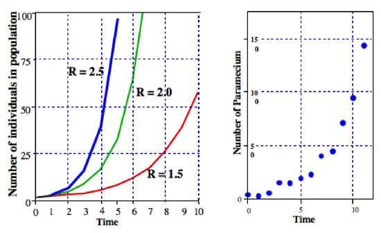
Growth in the size of a population (or other entity) in which the rate of growth increases as the size of the population increases is know as exponential growth. To model this growth we use the below formula, where (N(0)) = initial population size, and (N(t)) =  the projected population size (t is an arbitrary time): 

  N(t)= N(0)R 

The figure (above) depicts how rate (R) affects population size, when estimating future growth, given we know what the population size is at t initial.

Geometric Growth Model

Geometric growth model (equation below) expands upon the exponential growth model by including time (t) as a variable.  Including time as a variable is important for species that have defined growth periods (e.g., breeding season).  For a more detailed description of how this equation is derived, visit this website.

N(t)= N(0)(R^t)

(Knowledge Library, Nature.com)

Density Dependence

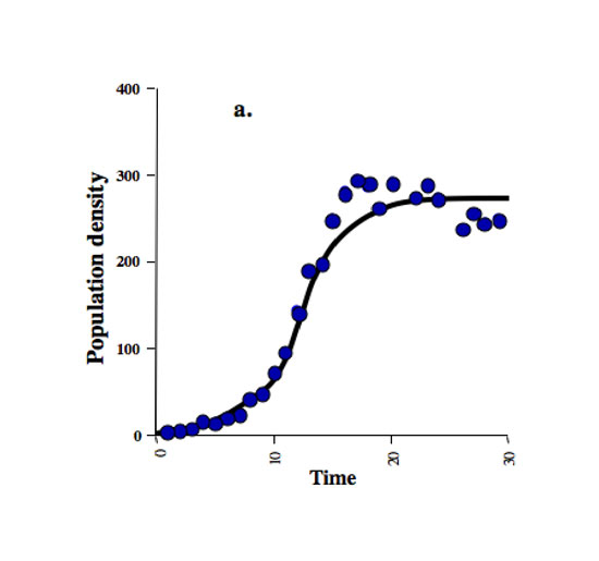
In the natural world, competition and resource availability limit population growth - this is described as carrying capacity (K).  That is, an environment or ecosystem is only able to support, or "carry", a maximum population size. As the population size approaches carrying capacity, the growth rate slows.  Population growth rate (R) is highest at the inflection point, where R=0.5.

Density dependent factors affecting population size, such as competition or predation are often biotic, whereas density independent limitations are often abiotic, such as environmental stress. 

Logistic Population Growth

This equation is density dependent, that is, as the population increases, intraspecific competition increases.  The logistic growth model is a common sigmoid curve or "S-shaped" curve, as seen in the carrying capacity graph above.   

(Knowledge Library, Nature.com)

To find the change in population size over time (dN/dt) while accounting for carrying capacity (K) we use the following equation ("Equation 8").  Where N = population size and r = rate of population change.   


Lotka-Volterra competition model

This model builds on the logistic growth model, by adding a competition coefficient, accounting for a species' ability to inhibit the growth of another (interspecific competition).  The equations below are the logistic growth model as discussed above for individual species (species 1, species 2), but a competition coefficient has been added. 

Competition coefficients may be denoted as alpha or beta, or as in this example, subscripts on the alpha are different.  This coefficient represents the degree to which their competitor may inhibit their growth (alpha) and the size of the competitor's population (N). 

 

(Townsend et al. 2008. Ecology)

(Knowledge Library, Nature.com)

 

Survivorship Curves & Life Tables

Through your field reports, you became very family with human life tables and survivorship curves.  However, if you need to review, these websites have an overview of life tables and survivorship (figure right).  

The Allee Effect, or Inverse Density Dependence at Low Density

This effect states that for certain species, when their population is at low densities, there is a positive relationship between population growth rate and density.  That is, decreased population growth is correlated with decreasing
abundance, which can result in the population's extinction.  This critical threshold (R=1), or Allee threshold, is the tipping point for a population's survival.

(Annual Reviews in Entomology, 2008)

The many factors that may lead to the Allee Effect have been loosely categorized as follows:

1. Genetic Inbreeding - leading to decreased fitness
2. Demographic Stochasticity (e.g., sex-ratio fluctuations, or low fecundity) 
3. Reduced intraspecific cooperation when densities are low

In practice, the Allee effect is of concern to conservation biologist.  Instances such as  managing rare species, monitoring species re-introductions, or preventing the establishment of non-native invasive species all  involve small population sizes.  

The most informative description I've found of this phenomenon online (and my source for information) is in this short article by Courcham et al. (1999) published in the scientific journal Trends in Ecology and Evolution (PDF link).